About:2D Thermal
2D Discretised Thermal Model for Cylindrical Cells - assess and design against cell hotspots and thermal gradients
Overview
About:2D Thermal is a discretised thermal model of a cylindrical cell, designed to accurately capture the temperature field within the main domains. The models are parameterised against test data and provide the cell temperature evolution over time as a function of heat generation rate, the boundary conditions applied to each cell face, and the external (sink) temperature.
Key features
- Compatible with any cylindrical battery model
Key applications
- Cell comparison and selection
- Determination of cooling system requirements
- Estimation of cell hotspots
- Estimation of cell thermal thermal gradients in high-rate applications such as fast charge
Technical Description
About:2D Thermal solves a two-dimensional heat equation for the temperature field of a cell, assuming axisymmetric heat transfer, internal heat generation, and cooling. Cooling is expressed using a user-defined lumped heat transfer coefficient on the different external faces of the cell. Local thermal heterogeneity of the cell is included, allowing the user to investigate the impact on heat transfer due to different axial and radial thermal conductivities.
Mathematical Specification

The 2D Thermal model is based around the primary constituents of a cylindrical cell, namely:
- Jelly-roll - The spirally wound electrode stack (anode, separator, cathode) that forms the core electrochemical structure of the cell.
- Can/Base - The cylindrical metal housing that encloses and protects the jelly roll while providing structural integrity.
- Cap - The top closure assembly that seals the can and typically integrates the electrical terminals and safety components.
Equations
The subscript \(m\) is used to specify a domain, where:
Assuming the structures inside the cell are perfectly cylindrical / annular, the cell geometries can be derived as:
The total cell heat source is divided into the three domains according to domain proportion \((f_m)\), and then applied uniformly:
Specific heat in each domain is linearly proportionally to temperature, which can be disabled by setting \(\frac{\partial {C_{p,m}}}{\partial T} = 0\):
Discretisation
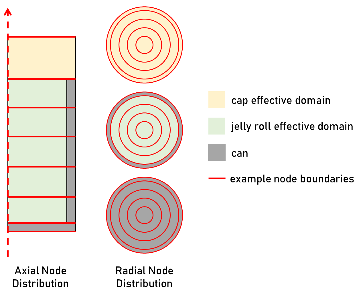
The separate domains are discretised further to form the nodal network model, as shown below. Some key points to note about the discretisation method:
- The battery core is represented as a cylindrical node, whilst surrounding nodes are concentric annuli. This arrangement is axially stacked into layers.
- The jelly roll domain is uniformly split into nodes of equal axial and radial thickness.
- The outermost node, surrounding the jelly roll, has a radial thickness (\(t_{r}\)) equivalent to the can thickness. This radial arrangement is consistent through the three distinct domains, even in layers consisting only of a single domain. This facilitates consistent heat transfer pathways between layers.
- The lowermost node layer (base), below the jelly roll, has an axial thickness (\(t_{z}\)) equivalent to the can thickness.
- The uppermost node layer, above the jelly roll, has has an axial thickness (\(t_{z}\)) equivalent to the cap height.
- The non-uniform nodes surrounding the jelly roll are only one node thick. All derivations used here assume an arbitrary number of nodes, with the assumption that the outer can and cap layers are always modelled as a single node thickness. Increasing \(N_r\) or \(N_z\) adds additional nodes to the jelly roll domain only. Eqs \ref{no_cannodes} & \ref{no_axnodes} must always be satisfied.
The following two equations define axioms used in the discretisation of the model, which must be satisfied for any size of nodal network.
\(N_{r}\) : Total number of radial nodes.
There is a single outer layer of radial can nodes \((N_{r\mathrm{,can}}=1)\), therefore:
\(N_{z}\) : Total number of axial node layers.
There is a single lower layer of axial can nodes \((N_{z\mathrm{,can}}=1)\), and a single upper layer of axial cap nodes \((N_{\mathrm{z, cap}}=1)\). Therefore:
Coordinate System
Nodal positions \((r_{i},z_{j})\) are defined at their geometric centre. These are required as several nodal properties are location-dependant, such as annulus volume, outer and inner radial areas. Additionally, these are used to form the temperature vs position output quantity.
These coordinates can be mapped to the node index \((i, j)\) by mathematical expressions, assuming that the previously defined domain structure and discretisation is retained. Where \(i=1\) at the battery core nodes, \(i=N_r\) at the circumference nodes, \(j=1\) at the base nodes, and \(j=N_z\) at the cap nodes.
Radial Coordinates, \(r_i\)
The distribution of nodes in the radial direction is shown in the Figure below. The central (core) node is cylindrical, surrounded by concentric annuli. Thus, the model has rotational symmetry around the cell centre \(z\) axis. This figure also lists the radial node centre coordinates as a function of visualisable geometric properties. The outer (can) node coordinate is easily determined from the can thickness.
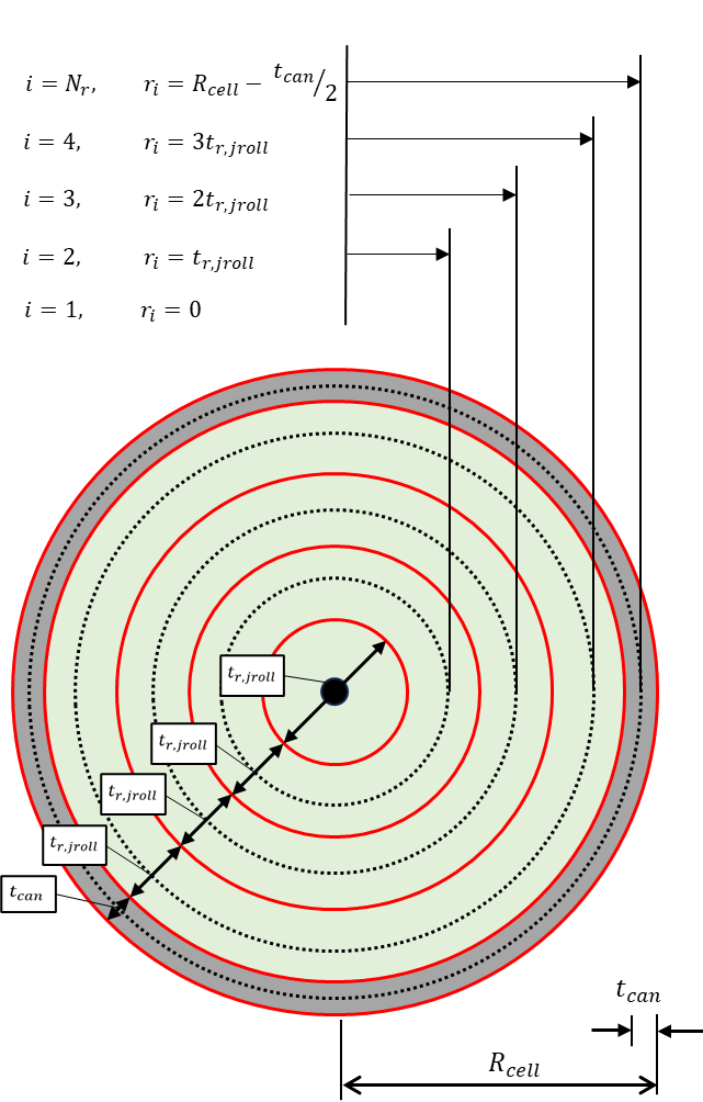
In the jelly roll domain, the nodes are uniformly distributed, with each having the same thickness, including the core node. The uniform jelly roll nodes are surrounded by a single outer node of thickness \(t_{\text{can}}\), representing the outer can. As shown in the above Figure, this radial arrangement is consistent throughout the thickness of the cell, even where the can is not modelled (E.G, the cap domain).
Each annular node has a node centre at the annulus radial midpoint. The central core node has a node centre at it’s centre point. The core node centre sets the the radial datum (\(r = 0\)) for the coordinate system.
Due to uniform annular node distribution in the jelly roll with cylindrical core node :
The full mathematical description of radial node thicknesses and centres are summarised in Eq \ref{t_full} and \ref{r_full}.
Axial Coordinates, \(z_j\)
The distribution of node layers in the axial direction is shown in the Figure below. In the jelly roll domain, the nodes are uniformly distributed, with each having the same thickness. The uniform jelly roll nodes are surrounded by a single base node layer of thickness \(t_{\mathrm{can}}\), and a single top node layer of thickness \(h_{\mathrm{cap}}\).
Each node has an axial node centre at the mid-thickness. The bottom of the cell sets the axial datum (\(z = 0\)) position for the coordinate system.
Note - derivations used here assume an arbitrary number of axial nodes layers, with the assumption that the top and base layers are always modelled as a single node thick. This satisfies Eq \ref{no_axnodes}. Increasing \(N_z\) adds additional axial node layers to the jelly roll domain only.
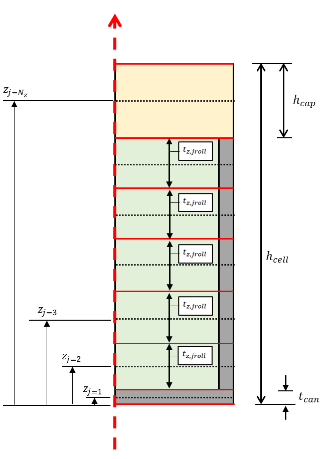
The mathematical expression of the base and cap axial node centre coordinates (\(z_1\) and \(z_{N_{z}}\)) are simply derived from the cell geometry, and shown in \ref{ax_pos}.
Looking at the internal (jelly roll) nodes in isolation, their node centre axial position from the beginning of the jelly roll is:
Where \(j_{\mathrm{jroll}}\) is the axial index of the node, beginning at the bottom of the jelly roll domain (rather than the base of the cell), and \(t_{z\mathrm{, jroll}}\) is the axial node thickness in the jelly roll domain. \(t_{z\mathrm{, jroll}}\) is determined for uniform node distribution in the jelly roll domain as:
Substituting Eq \ref{ax_pos} into Eq \ref{t_ax} and modifying the index system \(j\) to account for the base can node, results in:
The full mathematical description of axial node thicknesses and centres are summarised in Eq \ref{t_axial_full} and \ref{z_axial_full}.
Node Description
Surface Areas
Outer Radial Face Surface Area
General case \(\left( 1 \le i < N_r \right)\), \(\left( 1 \le j < N_z \right)\):
Inner Radial Face Surface Area
General case, annular node \(\left( 1 < i < N_r \right)\), \(\left( 1 \le j < N_z \right)\):
Special case, core node \(\left( i =1 \right)\), \(\left( 1 \le j < N_z \right)\):
Axial Face Surface Area
General case, annular node \(\left( 1 < i < N_r \right)\), \(\left( 1 \le j < N_z \right)\):
Special case, core node \(\left( i =1 \right)\), \(\left( 1 \le j < N_z \right)\):
Summary
Node surface area equations can be summarised as:
Other Evaluated Quantities
Volume:
Mass:
Heat generation [W]:
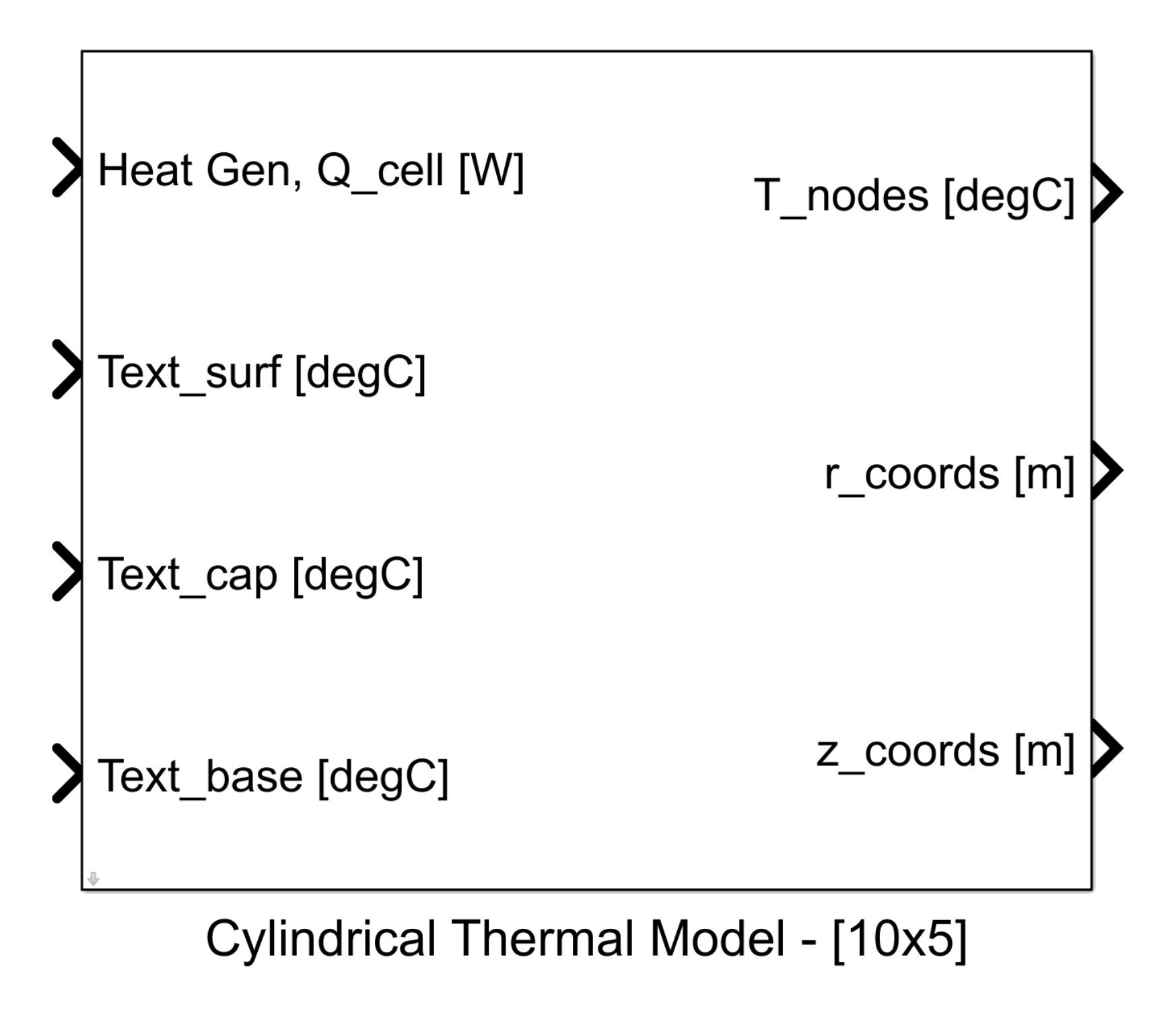
Simulink/Simscape Models
The About:2D Thermal Simscape implementation requires the following to be installed and licensed:
- MATLAB (R2021b or later)
- Simulink
- Simscape
The implementation comprises Simulink blocks provided in AE_therm_models_cyl.slx, which can be embedded in an application. Further documentation is provided internal to each block. See example_model.slx for an illustration of the coupling of a provided Simulink block to a user-defined model, including specification of operating conditions.
Version History
| Version | Release Date | Comments |
|---|---|---|
| 1.0 | 24 Nov 2025 | First release |