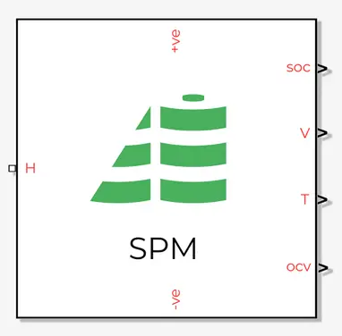
About:SPM
Single Particle Model - Efficient physics-based modeling that captures core electrochemical behavior
Overview
About:SPM is a physics-based model that represents the battery according to a set of physical equations and a corresponding parameter set. It is an implementation of the Single Particle Model (SPM), a simplification of the Doyle-Fuller-Newman model.
About:SPM predicts:
- Current-voltage relation
- Battery heat dissipation rate (excluding macroscopic Joule heating and mixing)
- Individual electrode overpotentials
- Lithiation distribution within active material particles (electrode-averaged)
About:SPM accounts for:
- State-of-charge (SOC)
- Temperature
- Charge-discharge hysteresis (at low C-rate)
- Rate capability (at low C-rate, according to physics-based loss computation)
- Cycling history (at low C-rate)
Key features
- Faster solution time than About:DFN or About:SPMe, but may be accurate only at low C-rate
- Compatible with any thermal model
- Compatible with distributed electronic networks and 3D cell/module/pack models
- Implements a subset of About:DFN, in which (as in About:SPMe), for each electrode, all active material particles are considered equivalent. Compared to About:SPMe, the model is further simplified by considering the electrolyte to be uniform throughout the cell, and by ignoring resistive losses in the electrolyte.
Key applications
- System prototyping for cell integration
- Representation of cell performance in 3D thermal models
- Degradation analysis*
* with provision of supplementary degradation data
Technical Description
About:SPM implements a single particle model, in which microscopic active material particle properties are described for a single representative spherical particle of a Li insertion material in each electrode. The particle response is then scaled to a cell response according to the relative proportions of active material in the two electrodes. All particles of a given material are assumed to have constant size and equivalent behaviour; particle size and shape distributions are not considered, and electrolyte resistance is ignored.
Li insertion rate and the corresponding faradaic current density is coupled according to a specified volumetric surface area to a microscopic 1D model, which solves the spherically symmetric Fick’s law diffusion equation to predict inserted Li concentration as a function of particle radius.
Internal heating is computed, including activation overpotential. Heat of mixing is ignored, to the first approximation. Temperature dependence of various physical quantities is accounted for by the specification of Arrhenius activation energies.
Mathematical Specification
The mathematical specification is an extension of the BPX standard (v0.3). The standard is extended for reasons of future-proofing, as itemised below:
- General values of activity multiplier \(1 + \partial \ln \gamma_\pm / \partial \ln c_l\) in (6). Defined = 1 identically by BPX.
- General values of transfer coefficient \(\alpha\) in (10) and (11). Defined = 0.5 identically by BPX.
Equations
Macroscopic dimension
The macroscopic dimension \(x\) is a 1D linear space \(0 \leq x \leq L_\mathrm{tot}\) and comprises successive regions with thicknesses \(L_\mathrm{neg}\), \(L_\mathrm{sep}\) and \(L_\mathrm{pos}\), where:
The macroscopic regions \(m=\mathrm{neg,pos}\) are defined as \(0\le x\le {{L}_{\text{neg}}}\) and \({{L}_{\text{tot}}}-{{L}_{\text{pos}}}\le x\le {{L}_{\text{tot}}}\).
In the macroscopic dimension:
For \(g_l = D_l,\kappa_l\):
The temperature dependence of any property \(g\) can be expressed as an Arrhenius relation:
Microscopic dimension
The microscopic dimension \(r\) is a 1D spherically symmetric space \(0 \leq r \leq r_{\mathrm{p},m}\) (\(m = \mathrm{neg, pos}\)). In this dimension:
Boundary Conditions
Initial conditions
Macroscopic boundaries
At the current collector boundaries (\(x = 0, L_\mathrm{tot}\)):
At the electrode—separator interfaces (\(x = L_\mathrm{neg},L_\mathrm{tot}-L_\mathrm{pos}\))
Macroscopic-microscopic coupling
At \(r = r_{\mathrm{p},m}\) in the microscopic dimension:
Loading conditions
The cell loading is specified by determining \(I_\mathrm{cell}\) from exactly one additional constraint for each discrete simulated time, chosen from the following options. Typically, the chosen loading condition will change at certain times during the protocol being simulated.
1 - Specified current:
2 - Specified voltage:
3 - Specified power:
Evaluated quantities
The cell heat source can be provided to a thermal model:
User Inputs: Operating Conditions
| Quantity | Unit | Description |
|---|---|---|
| \(I_\mathrm{app}\) | A | Applied current* |
| \(P_\mathrm{app}\) | W | Applied power* |
| \(\mathrm{SOC}_0\) | 1 | Initial state-of-charge |
| \(V_\mathrm{app}\) | V | Applied voltage* |
* Exactly one of the three possible applied quantities must be specified at each simulated time. Additional logic (for example, cut-off voltages or currents for different loading steps) can be built into the simulated protocol at the user’s discretion.
Internal Quantities
Supplied Parameterisation
All parameters are provided at the reference temperature except where otherwise indicated.
| Quantity | Unit | Description |
|---|---|---|
| \(A_\mathrm{el}\) | m\(^2\) | Active electrode area, per electrode pair |
| \(a_{\mathrm{vol},m}\) | m\(^{-1}\) | Active material volume fraction, electrode \(m\) |
| \(c_{l,0}\) | mol m\(^{-3}\) | Initial electrolyte concentration |
| \(c_{\mathrm{sat},m}\) | mol m\(^{-3}\) | Maximum (saturated) concentration of inserted Li, electrode \(m\) |
| \(D_l\) | m\(^2\) s\(^{-1}\) | Electrolyte diffusivity |
| \(D_{s,m}\) | m\(^2\) s\(^{-1}\) | Diffusivity, inserted Li, electrode \(m\) |
| \(E_{\mathrm{a},D_l}\) | J mol\(^{-1}\) | Activation energy, electrolyte diffusivity |
| \(E_{\mathrm{a},D_{s,m}}\) | J mol\(^{-1}\) | Activation energy, diffusivity, inserted Li, electrode \(m\) |
| \(E_{\mathrm{a},i_{0,m}}\) | J mol\(^{-1}\) | Activation energy, exchange current density, electrode \(m\) |
| \(E_{\mathrm{a},\kappa_l}\) | J mol\(^{-1}\) | Activation energy, electrolyte conductivity |
| \(i_{0,\mathrm{sat},m}\) | A m\(^{-2}\) | Exchange current density at 100% lithiated conditions, electrode \(m\) |
| \(L_q\) | m | Thickness, region \(q\) |
| \(N_\mathrm{el}\) | 1 | Number of electrode pairs |
| \(Q_\mathrm{nom}\) | Ah | Cell nominal capacity |
| \(r_{\mathrm{p},m}\) | m | Particle radius, electrode \(m\) |
| \(\Delta S_{m,0}\) | J K\(^{-1}\) mol\(^{-1}\) | Entropic coefficient, electrode \(m\) |
| \(T_\mathrm{ref}\) | K | Reference temperature |
| \(t_+\) | 1 | Transference number, Li+ in electrolyte |
| \(U_{m,0}\) | V | Open circuit potential vs Li+/Li at reference temperature, electrode \(m\) |
| \(V_\mathrm{EOC}\) | V | Cell upper (end-of-charge) cut-off voltage |
| \(V_\mathrm{EOD}\) | V | Cell lower (end-of-discharge) cut-off voltage |
| \(x_\mathrm{Li,neg,max}\) | 1 | Maximum lithiation extent, negative electrode at \(V = V_\mathrm{EOC}\) |
| \(x_\mathrm{Li,neg,min}\) | 1 | Minimum lithiation extent, negative electrode at \(V = V_\mathrm{EOD}\) |
| \(x_\mathrm{Li,pos,max}\) | 1 | Maximum lithiation extent, positive electrode at \(V = V_\mathrm{EOD}\) |
| \(x_\mathrm{Li,pos,min}\) | 1 | Minimum lithiation extent, positive electrode at \(V = V_\mathrm{EOC}\) |
| \(\alpha_m\) | 1 | Transfer coefficient, electrode \(m\) |
| \(\varepsilon_q\) | 1 | Porosity (electrolyte volume fraction), region \(q\) |
| \(\kappa_l\) | S m\(^{-1}\) | Electrolyte conductivity |
| \(\sigma_{\mathrm{eff},s,m}\) | S m\(^{-1}\) | Effective electronic conductivity, electrode \(m\) |
| \(\tau_q\) | 1 | Tortuosity, region \(q\) |
| \(1 + \partial \ln \gamma_\pm / \partial \ln c_l\) | 1 | Non-ideality coefficient |
Internal Variables
| Quantity | Unit | Description |
|---|---|---|
| \(c_l\) | mol m\(^{-3}\) | Electrolyte concentration |
| \(c_s\) | mol m\(^{-3}\) | Inserted Li concentration |
| \(f\) | V\(^{-1}\) | Inverse thermal voltage |
| \(D_{l,\mathrm{eff}}\) | m\(^2\) s\(^{-1}\) | Effective electrolyte diffusivity |
| \(i_\mathrm{far}\) | A m\(^{-2}\) | Current density, Li insertion |
| \(\mathbf{i}_l\) | A m\(^{-2}\) | Electrolyte current density |
| \(\mathbf{i}_s\) | A m\(^{-2}\) | Electric current density (electron-conducting phases) |
| \(i_\mathrm{v}\) | A m\(^{-3}\) | Volumetric current density, Li insertion |
| \(i_0\) | A m\(^{-2}\) | Exchange current density |
| \(\mathbf{N}_l\) | mol m\(^{-2}\) s\(^{-1}\) | Molar flux, electrolyte |
| \(\mathbf{N}_s\) | mol m\(^{-2}\) s\(^{-1}\) | Molar flux, inserted Li in particles |
| \(\mathbf{n}_r\) | 1 | Unit vector, outward normal direction, microscopic particle dimension |
| \(\mathbf{n}_x\) | 1 | Unit vector, outward normal direction, macroscopic dimension |
| \(Q_\mathrm{cell}\) | W | Cell heat source |
| \(Q_{\mathrm{max},m}\) | Ah | Maximum thermodynamic capacity in defined voltage window, electrode \(m\) |
| \(q_\mathrm{v,act}\) | W m\(^{-3}\) | Volumetric heat source, activation |
| \(q_\mathrm{v,JH}\) | W m\(^{-3}\) | Volumetric heat source, Joule heating |
| \(R_l\) | mol m\(^{-3}\) s\(^{-1}\) | Volumetric reaction rate, Li insertion |
| \(r\) | m | 1D spherical coordinate, microscopic particle dimension |
| \(t\) | s | Time |
| \(U\) | V | Open circuit potential vs Li+/Li |
| \(x\) | m | 1D linear coordinate, macroscopic dimension (current flow direction) |
| \(x_\mathrm{Li}\) | 1 | Lithiation extent |
| \(x_\mathrm{Li,surf}\) | 1 | Lithiation extent, active material particle surface |
| \(\eta\) | V | Overpotential |
| \(\kappa_{l,\mathrm{eff}}\) | S m\(^{-1}\) | Effective electrolyte conductivity |
| \(\phi_l\) | V | Electrolyte potential |
| \(\phi_s\) | V | Electric potential |
Variables inherited from thermal model
| Quantity | Unit | Description |
|---|---|---|
| \(T\) | K | Temperature |
Universal constants
| Quantity | Value | Description |
|---|---|---|
| \(F\) | 96485 C mol\(^{-1}\) | Faraday constant |
| \(R\) | 8.3145 J K\(^{-1}\) mol\(^{-1}\) | Gas constant |
Implementation Details
BPX JSON
The BPX JSON implementation consists of raw parameterisation data in a .json file compatible with the BPX v0.3 standard. These data are intended for use with a user-defined implementation of the equations in the Mathematical Specification.
The table below summarises the JSON paths that yield the variables specified above. Certain properties are derived from the BPX variables as indicated by the equations below:
Notes on JSON path equivalence
- Paths are given relative to the JSON element
Parameterisation, which is denoted.in relative paths below. - For properties defined by electrode, the string variable
{m}in{m} electrodeis to be substituted byNegativeorPositivefor negative or positive electrode properties respectively. - For properties defined by region, the string variable
{q}is to be substituted byNegative electrode,Positive electrode, orSeparator.
| Quantity | Unit | JSON Path |
|---|---|---|
| \(A_\mathrm{el}\) | m\(^2\) | ./Cell/Electrode area [m2] |
| \(a_{\mathrm{vol},m}\) | m\(^{-1}\) | ./{m} electrode/Surface area per unit volume [m-1] |
| \(c_{l,0}\) | mol m\(^{-3}\) | ./Electrolyte/Initial concentration [mol.m-3] |
| \(c_{\mathrm{sat},m}\) | mol m\(^{-3}\) | ./{m} electrode/Maximum concentration [mol.m-3] |
| \(D_l\) | m\(^2\) s\(^{-1}\) | ./Electrolyte/Diffusivity [m2.s-1] |
| \(D_{s,m}\) | m\(^2\) s\(^{-1}\) | ./{m} electrode/Diffusivity [m2.s-1] |
| \(E_{\mathrm{a},D_l}\) | J mol\(^{-1}\) | ./Electrolyte/Diffusivity activation energy [J.mol-1] |
| \(E_{\mathrm{a},D_{s,m}}\) | J mol\(^{-1}\) | ./{m} electrode/Diffusivity activation energy [J.mol-1] |
| \(E_{\mathrm{a},i_{0,m}}\) | J mol\(^{-1}\) | ./{m} electrode/Reaction rate constant activation energy [J.mol-1] |
| \(E_{\mathrm{a},\kappa_l}\) | J mol\(^{-1}\) | ./Electrolyte/Conductivity activation energy [J.mol-1] |
| \(K_m\) | mol m\(^{-2}\) s\(^{-1}\) | ./{m} electrode/Reaction rate constant [mol.m-2.s-1] |
| \(L_q\) | m | ./{q}/Thickness [m] |
| \(N_\mathrm{el}\) | 1 | ./Cell/Number of electrode pairs connected in parallel to make a cell |
| \(Q_\mathrm{nom}\) | Ah | ./Cell/Nominal cell capacity [A.h] |
| \(r_{\mathrm{p},m}\) | m | ./{m} electrode/Particle radius [m] |
| \(T_\mathrm{ref}\) | K | ./Cell/Reference temperature [K] |
| \(t_+\) | 1 | ./Electrolyte/Cation transference number |
| \(U_{m,0}\) | V | ./{m} electrode/OCP [V] |
| \(\partial U_m / \partial T\) | V K\(^{-1}\) | ./{m} electrode/Entropic change coefficient [V.K-1] |
| \(V_\mathrm{EOC}\) | V | ./Cell/Upper voltage cut-off [V] |
| \(V_\mathrm{EOD}\) | V | ./Cell/Lower voltage cut-off [V] |
| \(x_\mathrm{Li,neg,max}\) | 1 | ./Negative electrode/Maximum stoichiometry |
| \(x_\mathrm{Li,neg,min}\) | 1 | ./Negative electrode/Minimum stoichiometry |
| \(x_\mathrm{Li,pos,max}\) | 1 | ./Positive electrode/Maximum stoichiometry |
| \(x_\mathrm{Li,pos,min}\) | 1 | ./Positive electrode/Minimum stoichiometry |
| \(\alpha_m\) | 1 | Not specified. 0.5 by BPX standard definition. |
| \(\varepsilon_q\) | 1 | ./{q}/Porosity |
| \(\kappa_l\) | S m\(^{-1}\) | ./Electrolyte/Conductivity [S.m-1] |
| \(\sigma_{\mathrm{eff},s,m}\) | S m\(^{-1}\) | ./{m} electrode/Conductivity [S.m-1] |
| \(\mathcal{B}_q\) | 1 | ./{q}/Transport efficiency |
| \(1 + \partial \ln \gamma_\pm / \partial \ln c_l\) | 1 | Not specified. 1.0 by BPX standard definition. |
PyBaMM
The PyBaMM implementation requires a Python environment supporting the dependencies listed in the provided requirements.txt.
All parameterisation data are provided in a BPX JSON format as described above, and are loaded into the PyBaMM ParameterValues object using the PyBaMM built-in method ParameterValues.create_from_bpx().
Literature References
- Doyle, M.; Fuller, T.F.; Newman, J. Modeling of Galvanostatic Charge and Discharge of the Lithium/Polymer/Insertion Cell. Journal of The Electrochemical Society 1993, 140, 1526-1533, doi:10.1149/1.2221597.
- Fuller, T.F.; Doyle, M.; Newman, J. Simulation and Optimization of the Dual Lithium Ion Insertion Cell. Journal of The Electrochemical Society 1994, 141, 1-10, doi:10.1149/1.2054684.
- Doyle, M.; Newman, J.; Gozdz, A.S.; Schmutz, C.N.; Tarascon, J.M. Comparison of Modeling Predictions with Experimental Data from Plastic Lithium Ion Cells. Journal of The Electrochemical Society 1996, 143, 1890-1903, doi:10.1149/1.1836921.
- Thomas, K.E.; Newman, J.; Darling, R.M. Mathematical Modeling of Lithium Batteries. In Advances in Lithium-Ion Batteries, van Schalkwijk, W.A., Scrosati, B., Eds.; Kluwer Academic/Plenum Publishers: New York, 2002; pp. 345-392.
Version History
| Version | Release Date | Comments |
|---|---|---|
| 1.0 | 14 Mar 2023 | First release |