About:ECM
Equivalent Circuit Model - fast, accurate voltage prediction for accelerated pack concept design
![]()
Overview
Key features
About:ECM is an Equivalent Circuit Model (ECM) representing a battery as a network of electronic components. This model predicts the battery current-voltage relation as a function of state-of-charge (SOC) and temperature. Battery properties depend on State-of-Health (SOH), as defined by inputs for capacity fade and resistance increase. The model is capable of evaluating battery heat dissipation rate and battery temperature change in conjunction with a 0-dimensional lumped thermal model.
Features of About:ECM include:
- Compatibility with any About:Energy thermal model
- Compatibility with distributed electronic networks and 3D cell/module/pack models
- Compatibility with user-defined inputs for capacity fade and resistance increase
Key applications
About:ECM provides fast, accurate estimation of a single set of cell states (voltage, temperature, etc.) - typically representing a single battery cell (or scaled into an averaged representation of multiple cells or packs). It is fast enough to run numerous instances simultaneously, allowing prediction of distributed behaviour across battery packs.
About:ECM applications include:
- Cell comparison and cell selection
- Rapid system prototyping
- Beginning-of-life and aged-cell scenario analysis
- Analysis of battery pack variance and fault states
- Generation of heat generation rates for 3D thermal model inputs
Technical Description
About:ECM solves Kirchhoff's laws for the current-voltage relation as applied to a network of electronic components. About:ECM is compatible with any specification of current, voltage or power load on the battery. The About:ECM consists of the following:
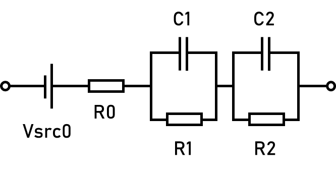
Figure 1: Schematic of a 2-RC pair circuit.
Open Circuit Voltage (OCV)
OCV represents the equilibrium voltage of a cell when no current flows and all transient effects have settled. This voltage directly reflects the thermodynamic potential difference between the positive and negative electrodes at a given state of charge. OCV varies nonlinearly with state of charge and temperature, serving as the fundamental voltage source in the equivalent circuit model.
Series Resistance (R0)
The series resistance captures the instantaneous voltage drop that occurs when current begins to flow through the cell. R0 causes an immediate voltage change proportional to the applied current, with no time delay, making it responsible for the sharp voltage discontinuity observed when switching between charge, discharge, and rest conditions.
Resistor Capacitor (RC) Pairs
RC pairs model the time-dependent voltage relaxation processes within the cell, capturing phenomena such as charge transfer kinetics and diffusion limitations. The resistor determines the magnitude of the voltage response, while the capacitor controls how quickly this voltage builds or decays, creating the characteristic curved voltage response observed during current steps or after current interruption.
A 2-RC pair circuit is the standard implementation within About:ECM - this provides a good resolution across multiple timescales within a cell, whilst mitigating risks of over-fitting and excessive complexity of parameterisation, along with maintaining a fast-executing simulation.
Mathematical Specification
Equations
Circuit Solution
The electrical circuit is defined with nodes \(k = 1, 2, ...\) including the special nodes "grd" and "term" which connect to the external load and between which total cell voltage is measured.
An electric potential \(\phi\) is defined at each node.
Circuit ground is defined:
Cell voltage is defined:
For a circuit with nodes \(k\) connected by components \(m\), Kirchhoff's laws require the currents \(I_m\) and voltages \(V_m\) to obey, for all \(k\) and all \(m\) respectively:
Cell current \(I_\mathrm{cell}\) is defined as positive in the charging direction. The quantities \(\theta_{km}\) represent the component connectivity. The following relationships apply at component level:
Component type OCV (open-circuit voltage source):
Component type R (resistor):
Component type C (capacitor):
The standard connectivities for the RC pair circuits are then as follows. \(\theta_{km}=0\) except where otherwise specified.
| \(m\) | \(k\) for which \(θ_{km} = -1\) | \(k\) for which \(θ_{km} = +1\) |
|---|---|---|
| OCV | grd | 1 |
| R0 | 1 | 2 |
| R1 | 2 | 3 |
| C1 | 2 | 3 |
| R2 | 3 | term |
| C2 | 3 | term |
The case of a 1-RC pair circuit is defined using the following substitutions in place of (6) and (7):
State of Charge (SOC)
The cell state-of-charge (SOC) evolves as follows:
The multiple of 3600 converts the unit of \(Q_\mathrm{nom}\) from A h (conventional reporting standards) to A s = C. \({\lambda}_{\mathrm{deg},Q}\) is a scalar degradation factor that can be specified by the user to simulate the cell with a degraded capacity.
SOC values reported in parameterisation are referenced to a condition of SOC = 1, corresponding to the cell state at nominal temperature 25 \(^\circ\)C following a long hold at the upper (end-of-charge) cut-off voltage \(V_\mathrm{EOC}\). Any other SOC is defined according to a relative charge passed, according to (13).
Degradation & State of Health (SOH)
Resistances and capacitances are determined from the provided lookup tables for beginning-of-life properties as \(f_{m,0}(T,\text{SOC})\) as below, where \(f\) represents a resistance \(R\) or capacitance \(C\) and \({\lambda}_{\mathrm{deg},m}\) is a component-specific degradation factor.
$$
\begin{equation} f_m = \lambda_{\mathrm{deg},m} f_{m,0}(T,\mathrm{SOC})
\label{resistance_deg}
\end{equation}
$$
Resistance increase is approximated as applying exclusively to the series resistance R0, which corresponds principally to ohmic and activation overvoltages of the cell. Thus:
No degradation correction is applied to the source voltage \(E_\mathrm{OCV}\), whose functional relation \(f(T,\mathrm{SOC})\) is assumed to be independent of degradation. Note, however, that capacity fade will influence the relation of SOC to charge passed (see below).
Hysteresis Effects
Optionally, a "one-state" hysteresis model is used, where the hysteresis state \(h\) is the solution to a relaxation equation according to a decay rate \(\gamma\):
Where:
Heat Generation
Heat generation is evaludated as the sum of three consituent parts:
- Irreversible Heat Generation
- Hysteresis Heat Generation
- Reversible Heat Generation
Irreversible Heat Generation
Also often referred to as \(I^2 R\), irreversible processeses are often the primary source of heat generation in battery cells, resulting from electrical resistance within the cell's components - electrodes, electrolyte and current collectors.
As current flows through these components, resistance causes heat generation which cannot be recovered - similar to resistive heating across a simple conductor.
Resistive heat scales with the square of current, making this mechanism particularly significant during high-rate charging or discharging operation.
Hysteresis Heat Generation
Hysteresis heat arises from the voltage gap between charging and discharging processes at the same state of charge. This phenomenon reflects the additional energy required to overcome thermodynamic barriers during lithium insertion and extraction from electrode materials.
While typically smaller than irreversible heat, hysteresis losses become notable during continuous cycling and contribute to the overall thermal profile of the cell, particularly in certain battery chemistries where voltage hysteresis is more pronounced.
About:ECM defines the hysteresis \(\Delta V\) as the difference between the instantaneous cell OCV and the 'average' OCV between the charge and discharge branches, such that:
Where:
Reversible Heat Generation
Reversible heat is unique in that it can either heat or cool a battery cell - this mechanism stems from changes to the entropic states within the cell's electrode materials during intercalation and deintercalation processes. The linear dependence on current magnitude means that reversible heat is often significant (relative to irreversible heat) at lower C-rate applications.
The magnitude and sign of reversible heat varies with State of Charge and temperature, along with the direction of current flow. For instance, if reversible heating is positive during charging at a certain state-of-charge (SOC), it will be negative during discharging at the same SOC. Over a full charge-discharge cycle, the total reversible heat theoretically balances out to zero (when ignoring minor degradation contributions).
More specifically:
Boundary Conditions
Initial values
A specification is required for the initial state of the cell - this can be determined as an input of either State of Charge or OCV, with the remaining property calculated as a function (also dependent on the initial user-specified value of cell polarisation):
Or:
Additionally,
Loading conditions
The cell loading is specified by determining \(I_\mathrm{cell}\) from exactly one additional constraint for each discrete simulated time, chosen from the following options. Typically, the chosen loading condition will change at certain times during the protocol being simulated.
- Specified current
- Specified voltage
- Specified power
Internal Variables
All internal and inherited variables are expressed as functions of time (\(t\)).
| Quantity | Unit | Description |
|---|---|---|
| \(C_\mathrm{C1}\) | F | Capacitance (RC pair 1) |
| \(C_\mathrm{C2}\) | F | Capacitance (RC pair 2) |
| \(E_\mathrm{OCV}\) | V | Cell open-circuit voltage (apparent with hysteresis) |
| \(E_\mathrm{OCV,avg}\) | V | Cell open-circuit voltage (average without hysteresis) |
| \(h\) | 1 | Hysteresis state |
| \(I_\mathrm{cell}\) | A | Cell current |
| \(I_m\) | A | Current through component \(m\) |
| \(Q_\mathrm{cell}\) | W | Total cell heat source |
| \(Q_\mathrm{hys}\) | W | Cell heat source (irreversible heating from hysteresis) |
| \(Q_{IR}\) | W | Cell heat source (irreversible heating from apparent resistive losses) |
| \(Q_\mathrm{rev}\) | W | Cell heat source (reversible heating) |
| \(R_\mathrm{R0}\) | Ω | Series resistance R0 |
| \(R_\mathrm{R1}\) | Ω | Resistance (RC pair 1) |
| \(R_\mathrm{R2}\) | Ω | Resistance (RC pair 2) |
| \(\mathrm{SOC}\) | 1 | State-of-charge |
| \(t\) | s | Elapsed time |
| \(V_\mathrm{cell}\) | V | Cell voltage |
| \(V_m\) | V | Voltage across component \(m\) |
| \(θ_{km}\) | 1 | Helper variable for connectivity: |
\(= +1\) for node \(k\) at positive terminal of component \(m\) \(= -1\) for node \(k\) at negative terminal of component \(m\) else \(= 0\) | | \(\phi_k\) | V | Electric potential at node \(k\) |
Variables Inherited From Thermal Model
| Quantity | Unit | Description |
|---|---|---|
| \(T\) | K | Temperature |
Inputs
User Inputs: Operating Conditions
| Quantity | Unit | Description | Default |
|---|---|---|---|
| \(I_\mathrm{app}\) | A | Applied current* | - |
| \(P_\mathrm{app}\) | W | Applied power* | - |
| \(V_\mathrm{app}\) | V | Applied voltage* | - |
| \(h_0\) | 1 | Initial hysteresis state | 0 |
| \(\mathrm{SOC}_0\) | 1 | Initial state-of-charge | 1 |
| \({\lambda}_{\mathrm{deg},Q}\) | 1 | Capacity degradation factor (capacity fade) | 1 |
| \({\lambda}_{\mathrm{deg},R}\) | 1 | Resistance degradation factor (resistance increase) | 1 |
* Exactly one of the three possible applied quantities must be specified at each simulated time. Additional logic (for example, cut-off voltages or currents for different loading steps) can be built into the simulated protocol at the user's discretion.
Parameterisation Values
Details of how the supplied parameterisation is encoded for each implementation are given in Implementation Details.
The below parameters are supplied as functions of state-of-charge and temperature \(f(\mathrm{SOC},T)\) at cell beginning-of-life (BoL):
| Quantity | Unit | Description |
|---|---|---|
| \(C_\mathrm{C1,0}\) | F | Capacitance (RC pair 1), cell BoL, tabulated function of SOC / temperature |
| \(C_\mathrm{C2,0}\) | F | Capacitance (RC pair 2), cell BoL, tabulated function of SOC / temperature |
| \(E_\mathrm{OCV,ch}\) | V | Open-circuit voltage (charge branch), cell BoL, tabulated function of SOC / temperature |
| \(E_\mathrm{OCV,dch}\) | V | Open-circuit voltage (discharge branch), cell BoL, tabulated function of SOC / temperature |
| \(R_\mathrm{R0,0}\) | Ω | Series resistance R0, cell BoL, tabulated function of SOC / temperature |
| \(R_\mathrm{R1,0}\) | Ω | Resistance (RC pair 1), cell BoL, tabulated function of SOC / temperature |
| \(R_\mathrm{R2,0}\) | Ω | Resistance (RC pair 2), cell BoL, tabulated function of SOC / temperature |
| \(\Delta S\) | V K\(^{-1}\) | Cell entropic coefficient |
| \(\gamma\) | 1 | Open-circuit voltage hysteresis decay rate |
The below parameters are supplied as scalar quantities:
| Quantity | Unit | Description |
|---|---|---|
| \(Q_\mathrm{nom}\) | Ah | Cell nominal capacity |
| \(V_\mathrm{EOC}\) | V | Cell upper (end-of-charge) cut-off voltage |
| \(V_\mathrm{EOD}\) | V | Cell lower (end-of-discharge) cut-off voltage |
Parameter File
Each ECM issue is accompanied by a parameter file (AE_ECM_Params.mat), which is a MATLAB structure containing the raw parameterisation data used to numerically define the model. These data are intended for use with a user-defined implementation of the equations in the Mathematical Specification.
A lookup table for properties depending on state-of-charge and temperature is given in AE_ECM_Params/params. Columns are named in a header row, below which all rows are data rows. The lookup variables are given in the first two columns, and data are given in the subsequent columns.
| Quantity | Unit | Type | Column name |
|---|---|---|---|
| \(\text{SOC}\) | 1 | Lookup | SOC |
| \(T\) | \(^\circ\)C | Lookup | T_degC |
| \(E_\mathrm{OCV,ch}\) | V | Data | V_OCV_ch_V |
| \(E_\mathrm{OCV,dch}\) | V | Data | V_OCV_dch_V |
| \(R_\mathrm{R0,0}\) | Ω | Data | R_R0_Ohm |
| \(R_\mathrm{R1,0}\) | Ω | Data | R_R1_Ohm |
| \(C_\mathrm{C1,0}\) | F | Data | C_C1_F |
| \(R_\mathrm{R2,0}\) | Ω | Data | R_R2_Ohm |
| \(C_\mathrm{C2,0}\) | F | Data | C_C2_F |
| \(\gamma\) | 1 | Data | gamma |
| \(\Delta S\) | V K\(^{-1}\) | Data | dUdT |
Scalar properties are given in AE_ECM_Params/params. Columns are named in a header row, and there is one data row containing the values for each property:
| Quantity | Unit | Type | Column name |
|---|---|---|---|
| \(E_\mathrm{OCV,ch}\) | V | Data | V_OCV_ch_V |
| \(E_\mathrm{OCV,dch}\) | V | Data | V_OCV_dch_V |
Notes on use
- Consult carefully the definition of SOC given in (13), according to which the data should be used. Definitions of SOC may vary in other applications or standards.
- To support standard usage, lookup data for \(T\) are provided in units \(^\circ\)C, not K.
- Where coefficient data are not available for a given input combination, a NaN value is given in the corresponding row and column.
Simulink/Simscape Models
The About:ECM Simscape implementation requires the following to be installed and licensed:
- MATLAB (R2021b or later)
- Simulink
- Simscape
The implementation comprises Simulink blocks provided in ECM_Library.slx, which can be embedded in an application. Further documentation is provided internal to each block. See exampleModel.slx for an illustration of the coupling of a provided Simulink block to a user-defined model, including specification of operating conditions.
Version History
| Version | Release Date | Comments |
|---|---|---|
| 1.0 | 14 Mar 2023 | First release |
| 2.0 | 23 Aug 2024 | Addition of degradation-compatible inputs |
| 3.0 | 11 Apr 2025 | Addition of 1-state hysteresis |
| 4.0 | 8 Aug 2025 | Addition of entropic & hysteresis heat generation |